Optimization of Hamerly’s K-Means Clustering Algorithm: CFXKMeans Library

This publication describes the application of performance optimizations techniques to Hamerly’s K-means clustering algorithm. Starting with an unoptimized implementation of the algorithm, we discuss:
- Thread scheduling
- Reduction patterns
- SIMD reduction
- Unroll and jam
Presented optimizations aggregate to 85.6x speedup compared to the original unoptimized implementation.
Resulting implementation is packaged into a library named CFXKMeans with interfaces for C/C++ and Python. The Python interface is benchmarked using the MNIST 784 data set. The result for K=64 is compared to the performance of K-means clustering implementation in a popular machine learning framework, scikit-learn, from the Intel distribution for Python. CFXKMeans performed our benchmark tests faster than scikit-learn by a factor of 4.68x on an Intel Xeon processor E5-2699 v4 and 5.54x on an Intel Xeon Phi 7250 processor.
The CFXKMeans library has C/C++ and Python API and is available under the MIT license at https://github.com/ColfaxResearch/CFXKMeans.
![]() Colfax-Kmeans-Clustering-Optimization.pdf (365 KB)
Colfax-Kmeans-Clustering-Optimization.pdf (365 KB)
Table of Contents
- 1. K-means Clustering
- 2. Optimizations
- 2.1. Initial Implementation
- 2.2. Multi-threading: Scheduling
- 2.3. Multi-threading: Reduction
- 2.4. SIMD Reduction
- 2.5. Unroll and Jam
- 3. Benchmark Results
- 3.1. Hardware
- 3.2. Methodology
- 3.3. FLOP/s
- 3.4. MNIST Benchmarks
- 4. Conclusion
- Appendix A: K-means Clustering Algorithm
- A.1. Standard Algorithm
- A.2. Hamerly's Algorithm
- Appendix B. Unsuccessful Optimization Attempts
1. K-means Clustering
It is no secret that there has been an upsurge in the amount and accessibility of all types of data in the recent years. From the location of cell phones with GPS to images uploaded to social media, digitized data is generated at a tremendous rate. And with this increase in information capture, there is a growing interest in analyzing and exploiting the available data sets.
It is particularly difficult to analyze unclassified data. That is because many data analysis algorithms (e.g., support vector machines and convolutional neural networks) fall under the category of supervised learning, where the input training data must be classified. So, without a significant investment into the initial classification, usually done painstakingly by manually going through the data, these algorithms cannot be applied. On the other hand, unsupervised training does not require classification of the input and is useful when there is a lot of unclassified data to work with.
Clustering algorithms are a group of unsupervised machine learning techniques that do not require the data to be classified. These group the data vectors (classified or unclassified) into clusters based on some criterion. The K-means method is a popular clustering algorithm. Given an integer K, the objective of K-means clustering is to group the input data (feature vectors) into K clusters in a way that minimizes the variance of the data within the clusters with respect to the cluster centroids.
K-means clustering and its variants are used in a wide range of applications. For example, it can be used in market analysis for automated customer segmentation. In bioinformatics, the K-means algorithm is used for grouping genes to discover functionally related gene groups. Spherical K-means clustering, a variant of K-means clustering, has been used as a feature extractor for computer vision.
The algorithm for K-means clustering is a much-studied field, and there are multiple modified algorithms of K-means clustering, each with its advantages and disadvantages. But the focus of this publication is not the analysis of the various K-means clustering algorithms. Instead, the focus will be on the optimization of the algorithm’s implementation as a C++ code to achieve better computational performance on modern architectures.
In Section 2, we discuss the implementation and optimization of the K-means clustering algorithm introduced by Hamerly (see 1 and 2). Hamerly’s algorithm is also described in detail in Appendix A. In Section 3, we put our final implementation to the test. We compare its performance to the Python scikit-learn library implementation of the algorithm on a multi-core and a many-core computing platform, in double and single precision, for a range of values of K.
The final implementation of the algorithm described in this paper, published as the CFXKMeans library, is usable from C/C++ and Python. The open-source CFXKMeans library is available under the MIT license at http://colfaxresearch.com/cfxkmeans.
2. Optimizations
This section will demonstrate the initial K-means algorithm implementation and computational performance optimizations that were applied. Each optimization is accompanied by a description of how to apply it, then a discussion on why it is effective, and, finally, a benchmark to show its benefit.
Our benchmark methodology is described in Section 3. Performance reported in Section 2 was measured on Intel Xeon Phi processor 7250 with K=64, using single precision floating-point arithmetics. Later, in Section 3, we report additional benchmarks of the final optimized code on more platforms and with other parameter values. The data set for the analysis used throughout the paper is the Mixed National Institute of Standards and Technology (MNIST) 784 data set. The benchmarks in our work are presented as wall-clock time and floating-point operations per second (FLOP/s).
2.1. Initial Implementation
We are going to focus on Hamerly’s variant of K-means clustering algorithm. Details of the algorithm are not discussed in this section; instead, they are covered in Appendix A. This section contains cross-references to variables introduced in the Appendix for convenience.
The most computationally intensive part of the K-means clustering algorithm is the assignment phase, where each feature vector is assigned to the closest cluster centroid. With the standard algorithm (see Appendix A.1), the distance from each feature vector to each cluster centroid must be calculated. Hamerly’s algorithm introduces a clever bounds check to avoid computing distances for some of the feature vectors (see Appendix A.2). The remaining computation for vectors that cannot be skipped is still the main computational workload for large data sets. Therefore, the focus of this section will be on the distance computations that occur when the bounds check triggers a calculation.
Listing 1 shows the computations following the bound check. This corresponds to lines 22-31 in Algorithm 2.
// INFINITY defined in
// ...
for(long i = 0; i < n_vectors; i++)
  // ... bounds check ...
  DTYPE min        = INFINITY; // distance to closest centroid.
  DTYPE second_min = INFINITY; // distance to second closest centroid.
  int min_index;
  for(int j=0; j < k; j++)  {
    DTYPE dist = 0.0;
    for(int f=0; f<n_features; f++)
        dist+=(data[i*n_features+f]-centroids[j*n_features+f])*
               (data[i*n_features+f]-centroids[j*n_features+f]);
    if(min > dist) {
      second_min = min;
      min = dist;
      min_index = j;
    } else if(second_min > dist) {
      second_min = dist;
    }
  }
  if(min_index != assignment_[i]) {
    converged = false;
    member_counter[min_index]++;
    member_counter[assignment_[i]]--;
    for(int f = 0; f < n_features; f++) {
      member_vector_sum[min_index*n_features+f]     +=data[i*n_features+f];
      member_vector_sum[assignment_[i]*n_features+f]-=data[i*n_features+f];
    }
    assignment_[i] = min_index;
    upper_bounds[i] = std::sqrt(min);
  }
  lower_bounds[i] = std::sqrt(second_min);
Listing 1. Computing the two nearest centroids, and assigning to the closest.
Here DTYPE is a compiler macro set to either float or double. The variables used in Listing 1 are listed below with names used in Algorithm 2 in parentheses:
- n_vectors: Number of input feature vectors (N)
- k: Number of clusters (K)
- n_features: Number of features (F)
- converged: Condition for algorithm to exit (converged)
- min: Distance to closest centroid (dmin)
- min_index: index of the closest centroid (csecmin)
- second_min: Distance to second closest centroid (dsecmin)
The arrays used Listing 1 are shown below with names used in Algorithm 2 in parentheses:
- data: array of size N×F containing input feature vectors (x)
- centroids: array of size K×F containing cluster centroids (μ⃗)
- assignment: array of size K containing the assignment of the feature vectors (A)
- member_count: array of size N containing the number of vectors assigned to a cluster centroid (M)
- member_vector_sum: array of size K×F containing the vector sum of vectors assigned to a cluster centroid (C⃗)
- upper_bounds: array of size N containing upper bound distance to the closest cluster centroid (u)
- lower_bounds: array of size N containing lower bound distance to the second closest cluster centroid (l)
This initial implementation compiled with the Intel C++ compiler completed in 34.16±0.02 seconds (13.97±0.01 GFLOP/s).
Initially, only performance with the executable compiled by the Intel C++ compiler will be discussed.
2.2. Multi-threading: Scheduling
The first optimization is to implement multi-threading. Once again, only the assignment phase is discussed in this section because it is the most computationally intensive part. However, note that thread parallelism is also implemented in other parts of the code. The OpenMP parallel framework is used to implement thread parallelism. For an introductory tutorial on OpenMP, see this.
With the nested for-loop structure of assignment phase, the for-loop parallelism is a strong choice for the parallel pattern. There are two choices of the loop to parallelize: parallelize over feature vectors (i) or parallelize over the centroids (j). Generally, it is preferable to add thread parallelism to the outermost for-loops because there is an overhead associated with starting and ending an omp for region. Furthermore, for-loop parallelism usually favors loops with large iteration counts. And for practical application of K-means clustering, N » K. Therefore, we choose to parallelize the implementation over the feature vectors.
#pragma omp parallel for
  for(int i = 0; i < n_vectors; i++)
Unfortunately, adding parallelism in this way will introduce race conditions for the assignment update shown in Listing 1. This code contains several shared variables and arrays that multiple threads write to: converged, centroid_counter and member_vector_sum. To resolve the race conditions on these variables and arrays, a parallelization reduction pattern must be implemented.
To implement parallel reduction, each thread must get a private buffer for each of the problematic variables and arrays, and the local computations and modifications must be done on these thread-private buffers. Once all the work has been completed, the results in these thread-private buffers are combined and reduced (i.e., aggregated) into a single buffer in a thread-safe manner. For an introductory tutorial on race conditions and parallel reduction, refer to this paper.
Since its inception, OpenMP supports the reduction clause to automatically implement this pattern for scalar variables. This clause is applied to the omp parallel directive in this format:
reduction(operation: variable)
Here operation is the operator used to combine the results together (e.g., +, &, max, etc.) and variable is the name of the variable for reduction. We can use this functionality for resolving race condition on the scalar variable converged:
#pragma omp parallel reduction(&: converged)
The OpenMP 4.5 standard extends the reduction clause to arrays. However, at the time of this writing, the OpenMP 4.5 standard is relatively recent, and only the newest compilers support this feature. Furthermore, later in this section we will experiment with and compare several different reduction patterns. So, we implemented the reduction pattern explicitly for the two arrays. The listing below shows our implementation of reduction on member_vector_sum and member_counter.
#pragma omp parallel reduction(&: converged)
{
  bool update_centroid[k];
  T *delta_member_vector_sum[k][n_features];
  int *delta_member_counter[k];
  // Initialize the thread local variables... //
#pragma omp for
  for(int i = 0; i < n_vectors; i++) {
    // ... Working on the  thread local versions
    update_centroid[min_index] = true;
    delta_member_counter[min_index]++;
    delta_member_counter[assignment_[i]]--;
    for(int f = 0; f < n_features; f++) {
      delta_member_vector_sum[min_index*n_features+f]     +=data[i*n_features+f];
      delta_member_vector_sum[assignment_[i]*n_features+f]-=data[i*n_features+f];
    } // ...
  }
  // Reduction
  for(int i = 0; i < k; i++) {
    if(update_centroid[i]) {
#pragma omp atomic
      member_counter[i] += delta_member_counter[i];
      for(int j = 0; j < k; j++)
#pragma omp atomic
        member_vector_sum[i][j] +=
          delta_member_vector_sum[i][j];
    }
  }
}
Listing 2. Implementation of reduction using atomics.
Here, both delta_member_vector_sum and delta_member_counter are declared inside the parallel region, and both of these variables are thread-private arrays. After all the work has been completed, the OpenMP pragma atomic is used to safely combine all the thread-private results into a single master result. Note that both delta_member_vector_sum and delta_member_counter were initialized to 0 instead of to their respective shared arrays, and are used to store the deltas (changes) in the respective shared arrays.
This implementation now completes in 0.837±0.001 seconds (570.11±0.41 GFLOP/s) on our 68-core processor. Comparing to the base case, the parallel efficiency is 34.16/(68×0.837)≈0.60. Because this is the total wall-clock time of the full application, which contains serial portions like memory allocation, linear scaling is not expected. Nonetheless, as we will soon see, efficiency can be improved.
Some of the issues preventing good parallel scalability can be found by analyzing this implementation with the Intel VTune Amplifier XE tool. This tool uses performance event collection to detect hotspots and performance issues. The screenshot below the VTune analysis summary page for this implementation.
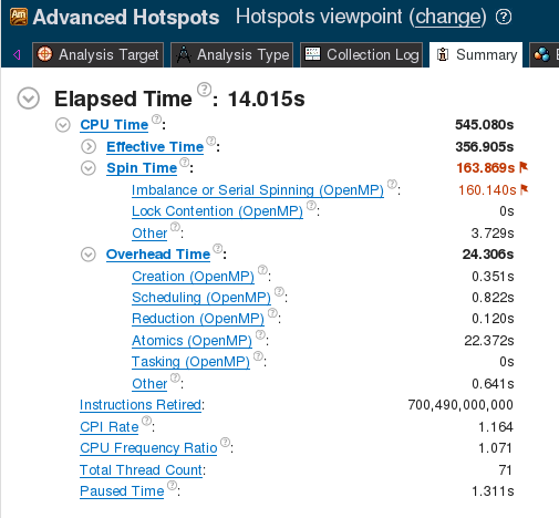
Figure 1. VTune Summary for linear reduction.
The large value of “Spin Time: → Imbalance or Serial Spinning” indicates that a significant portion of the computation time is wasted by idling CPUs.
Given the nature of the K-means clustering workload, a likely suspect for idling threads is workload imbalance. Workload imbalance occurs when some threads get more work than others. It is a common issue with parallel for-loops when there is variation in the amount of work inside each iteration. For Hamerly’s algorithm, the amount of work for each feature vector is variable. Some threads may get “lucky” and mostly receive feature vectors that are skipped, while others may get a large number of vectors that require the nearest centroid search. The result is that “lucky” threads will finish faster than others, and will idle until the “unlucky” threads finish their work.
The impact of the workload imbalance can be reduced by using a dynamic workload distribution. In dynamic workload distribution, iterations are distributed in small chunks (sets of iterations) and given to threads. When a thread has finished with the previously assigned chunk, it gets another chunk. Loop scheduling mode in OpenMP for-loops can be set using schedule clause, and there are two modes of scheduling with load balancing: dynamic and guided.
#pragma omp parallel for schedule(guided)
  for(int i = 0; i < n_vectors; i++) {
    // ... assignment phase ...
  }
With the guided distribution, the OpenMP scheduler hands out large sets of iterations at first. But as the number of remaining iterations decreases, the sets are made smaller and smaller until it reaches a minimum size. By default, the minimum chunk contains one iteration, but this value can be modified by adding a second argument to schedule:
#pragma omp parallel for schedule(guided, 10)
Both the schedule and the chunk size are tuning parameters, and we empirically found that the setting (guided, 10) performs the best. With the guided scheduling, the runtime drops to 0.731±0.001 seconds (652.8±0.5 GFLOP/s).
VTune analysis result, shown in the screenshot below (Figure 2), confirm a significant reduction in the spin time value.
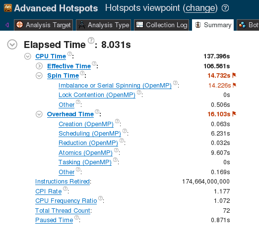
Figure 2. VTune Summary for Naive reduction.
2.3. Multi-threading: Reduction
In Figure 2, under the overhead time, VTune reports a fair amount of time spent on the atomic operation. Currently, an atomic pragma is used for every element inside the delta_member_vector_sum. With 68 threads, F=784 and K=64, this amounts to 68×784×64=3411968 atomic operations per while-loop iteration. Atomic operations are synchronization events, so they partially serialize the calculation. The number of synchronization events can be decreased to 68 (the number of threads) by using a critical region instead, as shown in the listing below.
#pragma omp parallel reduction(&: converged)
  {
    // ... assignment workload
    // Reduction
#pragma omp critical
    for(int i = 0; i < k; i++) {
      if(update_centroid[i]) {
        member_counter[i] += delta_member_counter[i];
        for(int j = 0; j < k; j++)
          member_vector_sum[i][j] +=
            delta_member_vector_sum[i][j];
      }
    }
  }
Listing 3. Implementation of reduction using critical.
Critical sections are also synchronization events, and they carry a greater overhead than atomic operations. However, for large values of F×K, the reduction in the number of synchronization events pays for the increased per-event overhead. This optimization reduces the execution time to 0.715±0.001 seconds (667.39±0.84 GFLOP/s).
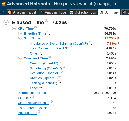
Figure 3. VTune Summary for critical reduction.
Even though this is an improvement, this code is still far from an ideal solution. Although there are fewer synchronization steps, the critical pragma allows only one thread at a time to work on the reduction code inside it. Thus, this reduction implementation is effectively single-threaded.
Another possible implementation is recursive reduction, where the results of individual threads are combined in pairs. Because each result pair can be combined independently of other results, this workload can safely be threaded without atomics. The advantage of this method is that it is a parallel reduction that does not have to rely on mutexes (atomics or critical sections). The recursive reduction, unfortunately, did not help the performance on the Xeon Phi system. The performance was 0.762±0.001 seconds (626.22±0.82 GFLOP/s). Although there are no mutexes, there is still a necessity to synchronize threads at every thread fork or join point. The details of this implementation are skipped in this publication because it does not add to the discussion in this section.
Finally, there is yet another reduction algorithm that allows us to avoid synchronization entirely. For this algorithm, instead of a thread-local buffer, a global buffer for delta_member_vector_sum and delta_member_counter must be created. With this global buffer, first consider the serial reduction implementation as shown below.
const in n_thread = omp_get_max_threads();
bool update_centroid_glob[n_thread][k];
T *delta_member_vector_sum_glob[k][n_features];
int *delta_member_counter_glob[k];
#pragma omp parallel reduction(&: converged)
{
  // ... Working on the assignment w/ global buffers
}
// Sequential Reduction
for(int tid = 0; tid < n_threads; tid++)
  for(int i = 0; i < k; i++)
    if(update_centroid_glob[tid][i]) {
      member_counter[i] += delta_member_counter_glob[tid][i];
      for(int j = 0; j < k; j++)
        member_vector_sum[i][j] +=
          delta_member_vector_sum_glob[tid][i][j];
    }
With this reduction, note that the data location written to in member_counter and member_vector_sum is different for each i. Therefore, it is safe to add multi-threading across the for-loop in i. To make this efficient, we switch the order of loops to move the for-loop in i outside, and then parallelize the i-loop as shown below.
// Parallel Reduction
#pragma omp parallel reduction(&: converged)
{
  // ... Working on the assignment w/ global buffers
#pragma omp for
  for(int i = 0; i < k; i++)
    for(int tid = 0; tid < n_threads; tid++)
      if(update_centroid_glob[tid][i]) {
        member_counter[i] += delta_member_counter_glob[tid][i];
        for(int j = 0; j < k; j++)
          member_vector_sum[i][j] +=
            delta_member_vector_sum_glob[tid][i][j];
      }
}
This implementation performs the reduction in parallel without any synchronization constructs. Of course, this method is not without drawbacks. In cases where the number of threads is larger than K, there are too few work items to keep all threads occupied. When K is small, this implementation performs worse than the implementation algorithms discussed above due to insufficient parallelism.
Empirically, this was the best method for K≤16 for Intel Xeon Phi processors with the MNIST data set. For smaller values of K, the application completed too quickly to get an accurate measurement. With the K=64 the execution time is now down to 0.628±0.001 seconds (759.84±0.85 GFLOP/s). This corresponds to parallel efficiency of ≈34.162/(68×0.628)=0.80, which is a 0.2 improvement from the initial reduction implementation.
Once again, this efficiency is calculated from the total-time that contains serial operations like initialization. To get an estimate for the efficiency of the parallelized assignment phase, this phase was timed separately.
double par_time = 0.0;
while(!converged) {
  // ...
  double par_start = omp_get_wtime();
#pragma omp parallel reduction(&: converged)
  {
    // ... Working on the assignment w/ global buffers
  }
  par_time += omp_get_wtime() - par_start;
  // ...
}
Here omp_get_wtime() is a microsecond-precision timer built into OpenMP. The initial implementation takes 33.98±0.02 for this part, whereas the new implementation gets 0.595±0.001. So the parallel efficiency just for this section is 33.98/(68×0.595)≈ 0.84. Although still not linear scaling, this is relatively good efficiency considering the unbalanced workload and the need for reduction.
2.4. SIMD Reduction
So far we have only discussed performance obtained with the Intel C++ compiler. Unfortunately, the last implementation takes 9.659±0.001 seconds (49.40±0.00 GFLOP/s) with the GNU compiler. One of the main reasons for this large discrepancy between the performance with Intel compilers and GCC is the lack of vectorization.
As discussed earlier, the code shown in Listing 1 is the largest contributor to the runtime for the K-means clustering workload. More precisely, the for-loop in f is the most computationally intense part of the code. Unfortunately, this loop has a vector dependency on dist, because all SIMD lanes are trying to modify dist at once. A technique called SIMD reduction must be implemented to remove this dependency. SIMD reduction is similar to reduction across threads. Instead of having a private variable for each thread, SIMD reduction creates a private “variable” for each SIMD lane. Intuitively, this can be thought of as having an array the same size as the vector register so that there is a memory location for each of the SIMD lanes. Once all the vector computations are complete, the contents of this array can be reduced into a scalar result.
The Intel C++ compiler automatically deals with this type of dependency and vectorizes the loop. GCC does not automatically vectorize a for loop when it detects this issue. Instead, it implements scalar computation. OpenMP 4.0 introduced the SIMD reduction clause that must force the compiler to implement this reduction. Its syntax is described below.
for(int j=0; j < k; j++)  {
  T dist = 0.0;
#pragma omp simd reduction(+: dist)
  for(int f=0; f<n_features; f++)
      dist+=(data[i*n_features+f]-centroids[j*n_features+f])*
              (data[i*n_features+f]-centroids[j*n_features+f]);
  // ... finding the closest ... //
}
Any compiler that is compliant with OpenMP 4.0 (such as GCC or Intel Compilers) will be able to vectorize loops with this type of dependency. However, it is important to note that how the reduction is implemented is up to the compiler implementation. The code below shows the GCC compiled assembly of the distance computation with the reduction clause:
## ... computation ... ##
        vmovups (%rsi,%r8), %zmm1           # loading the next set
        vsubps  (%rdx,%r8), %zmm1, %zmm1    # subtraction
        vfmadd231ps     %zmm1, %zmm1, %zmm0 # FMA

## ... Reduction ... ##
        vpxord  %zmm0, %zmm0, %zmm0         # setting 0th vector register to zero
        vaddss  -112(%rbp), %xmm0, %xmm0    # scalar add of first element
.LVL126:
        vaddss  -108(%rbp), %xmm0, %xmm0    # adding the second element
## .... adding elements 3 to 15 ... ##
.LVL140:
        vaddss  -52(%rbp), %xmm0, %xmm0     # adding the sixteenth (last) element
Listing 4.Assembly code of OpenMP SIMD reduction implementation with GCC.
An alternative to adding the SIMD pragma for the GNU compiler is to add the compiler flag -ffast-math. This will enable automatic vectorization for reduction, so long as automatic vectorization is switched on.
Finally, even though either method enables reduction vectorization, the best performance is achieved when both the compiler flag and the OpenMP pragma are present. Adding the reduction pragma and flag increases GCC performance, and it completes in 1.013±0.000 seconds (471.06±0.14 GFLOP/s). There was no change in the performance with the Intel C++ compiler as the reduction had already been vectorized automatically.
With the SIMD reduction, the code produced with the Intel C++ compiler is still faster, but the difference is not as drastic. There are a few reasons for the difference, one of which is that the Intel compiler implements a better reduction algorithm than the GNU compiler.
2.5. Unroll and Jam
The final optimization is applying unroll and jam, also known as register blocking. Unroll and jam is a loop transformation designed to increase vector register reuse. In order to apply unroll and jam, the code needs to have at least two nested for-loops. First strip-mine one of the outer for-loops, then move the new loop and make it the inner most for-loop. Finally, unroll the new innermost loop. The listing below demonstrates the unroll and jam transformation for dummy workload where vector B is added to each row in matrix A.
  // Original
  for(int i=0; i < N; i++)
    for(int j=0; j < N; j++)
      A[i][j] += B[j];
  // Strip-mine and permute
  for(int ii=0; ii < N; ii+=TILE)
    for(int j=0; j < N; j++)
      for(int i=ii; i < ii+TILE; i++)
        A[i][j] += B[j];
  // Unroll
  for(int ii=0; ii < N; ii+=TILE)
    for(int j=0; j < N; j++)
      A[ii+0][j] += B[j];
      A[ii+1][j] += B[j];
      A[ii+2][j] += B[j];
      // ... repeat to TILE
Listing 5. Implementing unroll and jam.
The unroll and jam optimization increases the reuse of vector register contents. In the above example, each vector loaded for B[j] is reused TILE times. Loading a vector register can take a number of cycles, especially if it needs to be loaded from high-level caches or system memory. This costly loading can be avoided if the loaded vector registers can be reused for multiple vectorized floating-point operations. The size of the TILE, or unroll factor, is a tuning parameter.
In some cases, this is done by the compiler as one of the automatic optimizations. And in other cases, the developer may need to use compiler directives or unroll by hand. Intel compiler has two pragmas, unroll and unroll_and_jam, that are designed for this use. However, we do not use them for two reasons. First, these compiler directives are not supported by GCC. And second, benchmarks have shown that the performance is better with manual unrolling.
To implement unroll and jam for the distance computations, the closest-two comparison from the j loop had to be separated. The listing below shows the implementation of the distance computation after unroll and jam.
  T dist_arr[k]; // container for the distances
  // initialize dist_arr
  const int kp_ = k - k%8;
  for(int jj=0; jj < kp_; jj+=8) {
#pragma omp simd reduction(+: dist_arr)
    for(int f=0; f<n_features; f++) {
      dist_arr[jj+0]+=(data[i*n_features+f]-centroids[jj*n_features+f])*
                       (data[i*n_features+f]-centroids[jj*n_features+f]);
      // ... dist1 to dist6 ... //
      dist_arr[jj+7]+=(data[i*n_features+f]-centroids[(jj+7)*n_features+f])*
                       (data[i*n_features+f]-centroids[(jj+7)*n_features+f]);
    }
  }
  // Remainder loop
  for(int j=kp_; j < k; j++)
    //  remaining dist computation

  for(int j=0; j < k; j++)
    //... finding the closest two and updating as needed ...
Listing 6. Implementing unroll and jam for the distance computations.
In the original implementation, the values data[i*n_features:f] are used for every iteration in i, so there are K×F/W vector loads, where W is the vector register width. With the unrolled implementation, the loaded values data[i*n_features:f] are reused eight times, so there are (K×F/W)/8 loads. Note that there is a separate remainder loop to deal with the last few iterations if K is not a multiple of 8. For the tuning parameter, the unroll factor of 8 was empirically found to give the best performance.
After the unroll and jam optimization, the executable with Intel Compiler completes in 0.408±0.000 seconds (1170±1 GFLOP/s). The GCC version completes in 0.678±0.001 seconds (704±1 GFLOP/s).
3>2.6. Optimization Summary
The figure below shows the performance for each optimization steps that were applied.
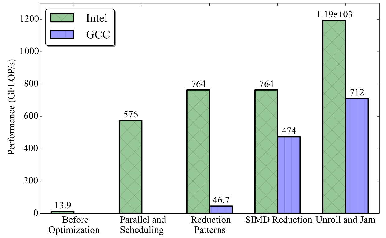
Figure 4. Performance at each of the optimization steps.
This wall-clock time performance includes initialization, allocation, and the serial computations (see Section 3). Because in this section we mostly discussed the optimization of the distance computation, it is also informative to study the time spent on just the distance computations. However, it is not trivial to compute the wall-clock time spent on the distance computation because the code is in a parallel region. Therefore, the average CPU-time (cpu_t) for this section of the code is computed instead.
double cpu_t = 0.0;
// ...
#pragma omp parallel reduction(&conversion) reduction(+: cpu_t)
  // ...
  T dist_arr[k]; // container for the distances
  const double t_start = omp_get_wtime();
  // ... dist computation ...
  cpu_t += omp_get_wtime();
  for(int j=0; j < k; j++)
    //... finding the closest two and updating as needed ...
With the current implementation, the average CPU-time per thread, given as cpu_t/num_threads, was 0.264±0.000 seconds. This time translates to 1808±1 GFLOP/s. This is by no means an accurate measure of performance because it ignores resource and lock contention. For example, consider an extreme case in which a similar analysis is done on a region that has omp critical. The actual wall-clock time will be much larger than the average CPU-time. This being the case, this metric was averaged over 10 runs and had a minuscule standard deviation. Therefore it is sufficient to give a rough estimate of the computational performance.
To put 1.8 TFLOP/s into perspective, the theoretical peak single precision performance of Intel Xeon Phi processor 7250 is 5.2 TFLOP/s. This is number is the product of the number of cores (68), the vector width in single precision (16), the throughput of the fused multiply-add instruction (2 instructions per cycle), the number of FLOPs in an FMA (2), and the AVX clock speed (1.2 GHz). Even though the base clock speed of the processor is 1.4 GHz, for heavy AVX-512 workloads, the frequency drops by 200 MHz to 1.2 GHz . For instructions other than pure FMA, the peak performance is lower. In our case, for each data element, there is a load instruction (loading centroid), a subtract instruction, and an FMA instruction. So 3 instructions are required to do 3 FLOPs. With 1 FLOP per instruction, the theoretical performance is 2.6 TFLOP/s. Even though 1.8 TFLOP/s is not far from this value, it is not close enough for us to believe the arithmetic performance is the bottleneck of our workload.
Another performance estimate gives us the insight into the bottleneck. The entire centroids data is read every time the nearest two centroids must be found for a feature vector. In the benchmarks used for Section 2, the centroids data is in single precision, K=4 and F=784. So the centroids data is 4×64×784 ≈ 200 KB in size. This is too large to fit in the L1 cache which is only 32 KB per core in size, so the centroids data is read from the L2 cache. To get the effective bandwidth of the distance computations, notice that for every data element in centroids array, there are 3 FLOPs (FMA and subtraction) that use this data element. Thus, for single precision, the conversion ratio from FLOPs to Bytes is 4/3 Byte/FLOP.
Using this conversion ratio and the 1.8 TFLOP/s from above, the approximate bandwidth is 2.4 TB/s.
Unfortunately, to the author’s best knowledge there is no documented measured peak bandwidth statistic for Intel Xeon Phi processors. Theoretically, the L2 cache on the Xeon Phi is capable of issuing 64-byte read per cycle (as discussed, e.g., in this book). Intel Xeon Phi processor 7250 has 34 L2 cache slices (one per tile) with a frequency of 1.4 GHz, so the theoretical peak bandwidth is 34×64 B×1.4 s-1=3 TB/s. 2.4 TB/s is very close to the theoretical peak value.
3. Benchmark Results
In this section, we test the fully optimized implementation on additional platforms for a range of values in K, in single and double precision. We also compare our performance to that of the popular scikit-learn library.
3.1. Hardware
Two processors were used in our benchmarks:
- Intel Xeon Phi processor 7250 with 16 GB of MCDRAM in quadrant mode with flat high-bandwidth memory and 96 GB of DDR4 memory at 2133 MHz in 16 GiB modules. The processor has 68 cores with 4-way hyper-threading and base clock speed 1.4 GHz.
- Intel Xeon E5-2699 v4 (formerly Broadwell) with 128 GB of DDR4 memory at 2400 MHz in 16 GB modules. The processor has 44 cores with 2-way hyper-threading clocked at 2.2 GHz.
3.2. Methodology
The K-means clustering workload was written as a C++ function. The executables used for the benchmarks were compiled with Intel Compiler 2017 update 2 and GCC 6.3.0. The following compiler flags were used for compilation.
> -ffast-math kmeans.cc
Our implementation, CFXKMeans, also provides a Python 2.7 module with a Python class wrapper that calls this C++ function. Because the performance of CFXKMeans is compared to that of the scikit-learn library later, all benchmarks were taken using the Python module version of CFXKMeans. For the same reason, the timing also included initialization costs, such as creating the buffers for the workload. The wall-clock time was measured using the Python time module with timers around the calls to K-means clustering function. For benchmarking, Intel Python distribution 2017 update 3 was used.
All benchmarks were taken with the same initial centroids. This is because the number of iterations required for convergence depends on the initial conditions, so different initial conditions would have led to different execution times. The timing was repeated 20 times, with the last 10 iterations reported. This is to avoid including hardware initialization costs like CPUs waking up from a lower power state.
The listing below shows a snippet from the Python benchmark script.
from sklearn.cluster import KMeans
import numpy as np
from sklearn.datasets import fetch_mldata
import time
import cfxkmeans

k=64
mnist = fetch_mldata('MNIST original')
data = mnist.data.astype(np.float32)
# For consistent initial conditions
stride = math.ceil(data.shape[0]/k)+1
init = data[::stride,:]

# For CFXKMeans: repeated 20 times
start = time.time()
cfxkmeans.KMeans(k, init).fit(data);
stop = time.time()

# For sklearn: repeated 20 times
start = time.time()
KMeans(n_clusters=k, init=init, max_iter=10000).fit(data)
stop = time.time()
Listing 7. Python benchmarking script.
Finally, this listing demonstrates how the benchmarks were run.
% # For Xeon Phi processor
% export OMP_NUM_THREADS=68 # 1 thread per core % export OMP_PLACES=cores
% export OMP_PROC_BIND=spread
% numactl -m 1 python kmeans.py #Using MCDRAM
% # For Xeon processor
% export OMP_NUM_THREADS=88 # 2 threads per core % export OMP_PLACES=cores
% export OMP_PROC_BIND=spread
% python kmeans.py
Listing 8. Running the Python benchmarking script.
These settings achieved the best performance for both Intel Compiler and GCC versions or implementations, as well as for scikit-learn.
3.3. FLOP/s
When optimizing applications, it is often useful to have performance in terms of Floating OPerations per second (FLOP/s) to gauge how close an application is to the theoretical peak performance. It is often difficult to get the exact number of instructions used in a program, but for the purposes of optimization, it generally suffices to get an approximate value. With the K-means clustering algorithm, majority of the floating point computation happens when computing the distances between a feature vector and each centroid (see Listing 1).
The innermost for-loop (f-loop) is visited F×K times for all feature vectors that needed the distance computed (i.e. the if-branch was taken). Inside the f-loop, there are 3 floating operations (one of the subtractions is redundant). So the lower bound approximation of the number of FLOPs is 3×F×K×distcomp FLOPs, where distcomp is the number of distance computations that occurred. To get the FLOP/s performance, simply divide this number by the wall-clock time.
One important note is that the number of distance computation is sensitive to the precision of floating-point operations. Therefore, even though the final output was consistent between the hardware architectures, compilers, and optimizations, the value of distcomp was not. With that said, typically the difference was only one or two whereas the total was over a hundred thousand.
3.4. MNIST Benchmarks
The reported benchmarks were taken with the Mixed National Institute of Standards and Technology (MNIST) 784 database. The MNIST database was chosen because it is a well-studied and accessible data set with a large enough problem size that makes it practical for benchmarking. However, it should be noted that the K-means clustering method is not a practical approach to solving the hand-written digit classification problem presented by the data set. Thus, only the computational performance is reported in this section. Also, both the training data set and the test data set of the MNIST database was used for benchmarks.
For some data sets, K-means clustering analysis can be sensitive to the precision level due to its iterative nature. MNIST data-set happens to be such a data set. CFXKMeans gave identical results for both double precision and single precision on both Xeon processor and Xeon Phi processor. On the other hand, the scikit-learn library in the Intel Python distribution did not give identical results for Xeon Phi processor. As such, the double precision result on the Xeon processor was used as the verification value.
Both single and double precision performances were taken on Xeon Phi processor and Xeon processor. In each case, the performance for K⊂{16,32,64,128} were taken using three K-means clustering implementations: CFXKMeans (Intel Comp.), CFXKMeans (GCC) and scikit-learn (Intel). It should be noted that the benchmarks are not a true “apples-to-apples” comparison. scikit-learn uses a different variant of the K-means clustering algorithm: Elkan’s algorithm.
Publication by Hamerly reports that Elkan’s algorithm outperforms Hamerly’s algorithm for MNIST 784 with the values of K used in the benchmarks. Therefore, the author believes that the presented benchmarks are a fair comparison of the frameworks. Regardless, the results should be taken with a grain of salt, as the frameworks will behave differently for different data sets, initial conditions, and values of K. Typically, Elkan’s algorithm performs better for larger values of K while Hamerly’s algorithm performs better at lower values of K.
The tables below show the full benchmark results in wall-clock time for Xeon Phi processor and Xeon processor respectively.
| precision | k | CFXKMeans (IC) | CFXKMeans (GCC) | scikit-learn (Intel) |
|---|---|---|---|---|
| single | 16 | 0.115±0.000 | 0.133±0.000 | 0.841±0.045 |
| single | 32 | 0.199±0.001 | 0.263±0.001 | 1.477±0.103 |
| single | 64 | 0.411±0.001 | 0.678±0.002 | 2.270±0.086 |
| single | 128 | 0.554±0.001 | 0.981±0.001 | 3.332±0.093 |
| double | 16 | 0.170±0.000 | 0.203±0.000 | 1.384±0.010 |
| double | 32 | 0.310±0.000 | 0.421±0.000 | 2.506±0.027 |
| double | 64 | 0.776±0.001 | 1.126±0.001 | 4.105±0.168 |
| double | 128 | 1.199±0.003 | 2.132±0.024 | 3.554±0.095 |
Table 1.MNIST 784 performance on Xeon Phi processor in term of wall-clock time. Entries where Xeon Phi processor outperforms Xeon processor is in bold.
| precision | k | CFXKMeans (IC) | CFXKMeans (GCC) | scikit-learn (Intel) |
|---|---|---|---|---|
| single | 16 | 0.104±0.004 | 0.119±0.003 | 0.610±0.026 |
| single | 32 | 0.165±0.001 | 0.233±0.002 | 1.124±0.011 |
| single | 64 | 0.385±0.004 | 0.611±0.005 | 1.817±0.036 |
| single | 128 | 0.654±0.003 | 0.896±0.002 | 3.460±0.065 |
| double | 16 | 0.206±0.007 | 0.230±0.007 | 1.390±0.007 |
| double | 32 | 0.329±0.002 | 0.478±0.008 | 2.469±0.009 |
| double | 64 | 0.883±0.001 | 1.324±0.007 | 4.077±0.011 |
| double | 128 | 1.305±0.001 | 1.977±0.012 | 3.663±0.008 |
Table 2.MNIST 784 performance on Xeon processor in term of wall-clock time. Entries where Xeon processor outperforms Xeon Phi processor is in bold.
Xeon processor generally out performs Xeon Phi processor for single precision workloads, while Xeon Phi processor beats Xeon processor for double precision workloads.
In order to measure the speedup provided by these libraries, the base scikit-learn (i.e., main-branch) performance was measured for K=64 on the Xeon processor. The scikit-learn version used was 0.18.2, and taken with Python 2.7.5 [GCC 4.8.5 20150623 (Red Hat 4.8.5-4)]. Using the identical procedure and settings as for other two, main-branch Python completed in 30.071±0.089 seconds for single precision, and 66.766±0.202 seconds for double precision. Using this as the baseline, the relative speedup was computed for CFXKMeans and Intel Python. The figure below shows the relative speedup.
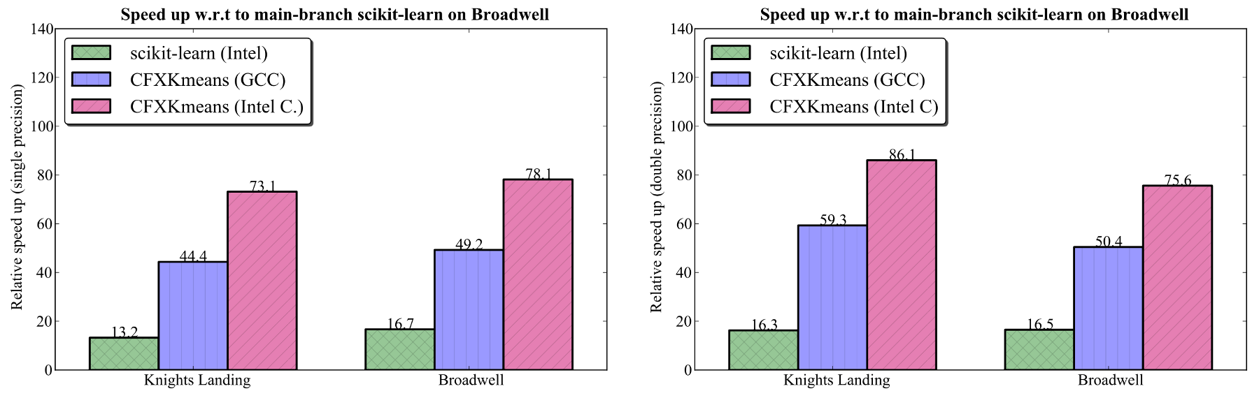
Figure 5. Relative speedup compared to main-branch scikit-learn on Broadwell (K=64). Left: single precision. Right: double precision.
4. Conclusion
We presented the optimization path and the final performance results of the CFXKMeans library, which contains a K-means clustering routine based on Hamerly’s algorithm.
In our benchmarks for the MNIST 784 data set, CFXKMeans performs approximately 5 times faster than the same routine from the scikit-learn library available with Intel distribution for Python. This speedup is observed on a 68-core Intel Xeon Phi 7250 processor and on a 44-core Intel Xeon E5-2697 v4 processor.
This publication pursued two goals. One was to serve as a practical guide for developers in the application of the discussed optimizations.
Another was to document the thought process behind the optimizations for potential future development of CFXKMeans.
This publication contains detailed analysis of the various optimizations that have been applied to the K-means clustering algorithm:
- detecting workload imbalance and resolving it with scheduling
- analyzing various parallel reduction algorithms
- SIMD reduction with OpenMP
- Re-using registers with unroll and jam.
Because we used the C++ language with OpenMP-compliant directives, our implementation is portable. We see high performance on Intel Xeon and Intel Xeon Phi processors. Furthermore, we expect that our optimization will work well on future models of Intel processors and on non-Intel architectures with similar design. That is because we targeted the fundamental building blocks of parallel processors: multiple cores, vector instruction support, and coherent hierarchical caches.
The product of this work, the CFXKMeans library, is available under the MIT license at https://github.com/ColfaxResearch/CFXKMeans.
Appendix A: K-means Clustering Algorithm
This section is a brief introduction to the K-means clustering algorithm.
The goal of K-means clustering is to take a set of feature vectors  and group them into K clusters
  so that the sum of variances within clusters is minimized:

Here  is the centroid of cluster
  , computed as the mean of the vectors assigned to it.
The standard algorithm for solving this workload was introduced in the 1960s, and is often referred to as Lloyd’s algorithm.
Various efforts have been made to improve on this standard algorithm.
In 2003 Charles Elkan introduced a new algorithm that is optimized for large values of K.
Then in 2010, George Hamerly introduced an algorithm that is optimized for smaller values of K.
CFXKMeans library uses the Hamerly’s algorithm for the K-means clustering, whereas scikit-learn uses Elkan’s implementation.
Though there have been further development in K-means clusterng algorithms, only the algorithms relevant to the paper will be described in this section: the standard algorithm first, followed by the Hamerly’s algorithm.
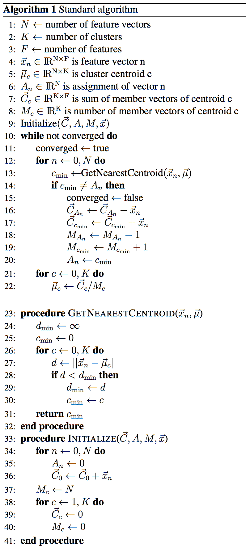
A.1. Standard Algorithm
Standard algorithm is an iterative algorithm to find the minimum variance clusters. It starts with initial “guesses” for the cluster centroids, and these centroids are refined at each step until the algorithm converges. K-means clustering algorithm convergence time strongly depends on these initial conditions. There are numerous studies on how best to select the initial guesses. However, this is beyond the scope of this discussion. In the benchmarks presented in the paper, “guesses” are selected from the feature vectors (input).
Each step can be divided into two phases: assignment and update.
- Assignment Phase:
Each feature vector (input) is assigned to the cluster that minimizes the variance. Because the Euclidean distance is the square root of the sum of squares, this is equivalent to assigning a feature vector to the closest cluster centroid. - Update Phase:
Each centroid is updated based on its current members. In other words, the centroid position is set to the vector average of the feature vectors assigned to it.
When there are no changes to the assignment in the assignment phase, then the algorithm has converged to the local minimum.
Standard algorithm is shown below.
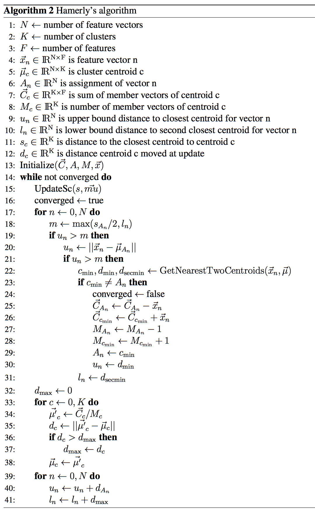
A.2. Hamerly’s Algorithm
In the standard algorithm (shown above), the most computationally intensive part is in GetNearestCentroid. This part is also often computationally wasteful because the nearest centroid often does not change between while-loop steps. Hamerly’s algorithm aims to reduce the number of wasted nearest centroid computations by introducing two light-weight conditions to see if the computation is required. Both conditions use the upper bound distance to the assigned centroid. In the subsequent discussion, let  be the upper bound of the feature vector
  to its assigned centroid.
The first condition takes advantage of the lower bound of distance to the second nearest centroid for each vector, which is denoted  for feature vector . Note that this lower bound does not specify which centroid is the potential second nearest centroid. It is the minimum distance that any non-assigned centroid can be from the feature vector. If the upper bound of distance to the assigned centroid, is less than , then the assigned centroid must be the closest centroid. Thus if
  , then the distance computations can be skipped because the assignment of vector cannot change.
The second condition uses the distance of the nearest centroid to the assigned centroid. Suppose vector is assigned to cluster centroid  , and nearest centroid to is
  . Triangle inequality gives us:


Now assume that  and substitute this in the left-hand side:
 - u_n \leq ||c_2-x_n||")

Note that for any other centroid  the distance
  will be larger and the above still holds. Thus, if
  , then the assignment does not change. For subsequent discussion let the distance to closest centroid for centroid
  be
be  .
.
These two conditions can be combined into ") where
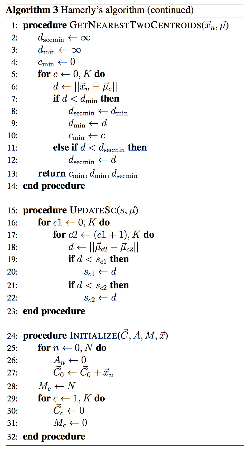
where  is the assignment of vector . If the condition fails, the algorithm first tightens the bound by re-computing . And if the condition fails again with the tightened bound, then the distances are computed. During the distance computation, the distances to the closest and the second closest clusters are stored and used to update both and .
Minimum cluster centroid distances, , can be computed at every step relatively cheaply, because the number of clusters,  , is typically small compared to the number of vectors in the data set. The values must be updated at every step as the assigned centroid may move, but it would be costly to compute the exact change in distance to the assigned centroid with respect to
  . Thus, the absolute maximum change in distance, which is the total distance that the assigned centroid moved, is added to . Similarly, must be updated as well. In this case, the maximum distance that any centroid moved is added because this is the lower bound distance to any centroid except the assigned one.
The pseudocode of Hamerly’s algorithm is shown below.
Appendix B. Unsuccessful Optimization Attempts
This section will discuss some of the unsuccessful optimizations that were attempted but did not result in a performance gain.
One attempted optimization was to reduce distance computation to a matrix-matrix multiplication. Let matrix  contain the
  feature vectors that require distance computations to centroids, with
  representing the
  -th vector row. And matrix
  contains the centroids, with
  representing the
  -th centroid row. Then the distance computation has the form:

where  is the distance squared between i-th feature vector and j-th centroid. This then can be reduced to:

_{ij} + | C_j |^2,")
where _{ij}") is the ij-th element in the matrix product
is the ij-th element in the matrix product  .
.
It is simple to pre-compute the  and
and  terms for all i and j, respectively. Thus the bulk of the computation becomes the matrix product
  . One important note, however, is that the matrix
  contains only the feature vectors that need distance computation, which is different between each while loop iteration. This means that has to be constructed every time from the original data array.
There are couple of benefits to reducing the problem to matrix product. Unlike the current bandwidth-bound implementation, matrix product is compute-bound and can achieve performance much closer to the theoretical peak performance. Furthermore, there are well established BLAS libraries, such as Intel MKL, that has already been optimized for matrix produce.
Although in practice, the performance was worse. Analysing on the work required to construct reveals why. Since feature vectors are copied, this is  elements that are read from and written to memory for copying from data into (2 reads, and 1 write for a factor of 3) then back afterwards (another factor of 2). On the other hand, the matrix product has
  floating point operations. This means that for each data element copied, there are
  floating operations on it. Using theoretical numbers for Xeon Phi, for every data read from memory takes as long as
  floating point operations. Thus, the value of must be extremely large to justify this copy. So in practice benefit from the improved computational performance of matrix product did not outweigh the lost performance to the copy.
The second optimization was to tile the distance computation in , just as for . This way, the centroid data can be reused on multiple iterations of instead of reading the entire data for every iteration. Unfortunately, the if statement check for the bounds prevents us from simply moving the tiled for-loop inside distance computation. To implement this, the code inside loop had to be split into two loops: the first will compile a list (std::vector) of indices that need distance computation, and the second will iterate through the list and perform the distance computations.
This is somewhat similar to the matrix product optimization. The matrix product optimization collected the needed feature vectors into matrix , whereas in this case only the indices of the needed feature vectors are collected.
Unfortunately, this optimization was also unsuccessful. Because several feature vectors are worked on at a time, and there is no guarantee that these feature vectors are close to each other in memory, the access pattern for the feature vector was that of a random access. Furthermore, the additional feature vector data means that there is even less space to work with in the L2.