HPLinpack Benchmark on Intel Xeon Phi Processor Family x200 with Intel Omni-Path Fabric 100

We report the performance and a simplified tuning methodology of the HPLinpack benchmark on a cluster of Intel Xeon Phi processors 7250 with an Intel Omni-Path Fabric 100 Series interconnect.
Our benchmarks are taken on the Colfax Cluster, a state-of-the-art computing resource open to the public for benchmarking and code validation. The paper provides recipes that may be used to reproduce our results in environments similar to this cluster.
![]() Colfax-HPL-Intel-Xeon-Phi-x200-and-Intel-Omni-Path-100.pdf (130 KB)
Colfax-HPL-Intel-Xeon-Phi-x200-and-Intel-Omni-Path-100.pdf (130 KB)
Table of Contents
- Section 1. HPLinpack Benchmark
- Algorithm
- HPL Configuration File
- Section 2. System Configuration
- Intel Architecture
- Colfax Cluster
- Section 3. Results
- Recipe
- Performance
- Impact of System Configuration
- Section 4. Summary
Section 1. HPLinpack Benchmark
The HPLinpack benchmark generates and solves on distributed-memory computers a large dense system of linear algebraic equations with random coefficients. The benchmark exercises the floating-point arithmetic units, the memory subsystem, and the communication fabric. The result of the HPLinpack benchmark is based on the time required to solve the system. It expresses the performance of that system in floating-point operations per second (FLOP/s).
To standardize the HPLinpack results, a code called HPL was developed. HPL is a software package implementing the HPLinpack benchmark. The code performs the benchmark workload and reports the timing and an estimate of the accuracy of the solution. HPL is portable because for linear algebra it interfaces with standard libraries, including the Basic Linear Algebra Subprograms (BLAS) and Linear Algebra Package (LAPACK), and uses the Message Passing Interface (MPI) for communication in a cluster. At the same time, optimized versions of HPL for particular architectures exist (e.g., Intel-optimized HPL) and can be used without compilation.
The HPLinpack benchmark expressed as HPL is an industry-standard test of floating-point capabilities of parallel high-performance computing systems. For instance, the TOP500 project provides a regularly updated list of the most powerful computer systems in the world ranked using HPL. The systems are ranked according to their maximum LINPACK performance achieved,  .
.
Algorithm
HPLinpack benchmark solves a system of linear algebraic equations of size  ,
,

The solution is obtained by first computing the LU factorization with row partial pivoting and then solving a triangular system of equations. The size of the problem,  , can be chosen arbitrarily. Usually, it is chosen to maximize the problem size while still fitting the application in the RAM of the compute nodes.
In order to verify the solution, the input matrix and the right-hand side are regenerated, and the normwise backward error is computed:
 n},")
where  is the relative machine percision. The solution is verified when the condition
 ") is satisfied, where
is satisfied, where ") is a threshold value of the order 1.0.
is a threshold value of the order 1.0.
To convert the execution time  to performance in GFLOP/s, the benchmark assumes that the number of floating operations performed to solve the system
  is
is  , i.e.,
^{-1}.")
HPL Configuration File
HPL gives the user the ability to tune the benchmark parameters and select one of multiple factorization algorithms. All benchmark arguments are read from a text file called HPL.dat. Tuning the parameters in this file for a particular system is often difficult and, in general, requires a scan of a parameter space. Instead of a parameter scan, we used a simplified tuning methodology. Specifically, we focus only on the most important arguments in this file: N, NB, P and Q, and use heuristic rules for picking their values.
Problem size
The amount of memory used by HPL is only slightly greater than the size of the coefficient matrix. To get the best performance of a system, you need to set the problem size to the maximum size that would fit into the memory of the computing system. If is chosen too small, the performance will be dominated by memory or network traffic, and the maximum performance of the system will not be demonstrated. If the problem size chosen is too large, performance will drop due to virtual memory swapping to the hard drives.
This expression is an estimate of the value of for a cluster comprising  compute nodes with each compute node having a memory of size
  :
:

where  is a “slack factor” no greater than 1.0. We used ≈0.9 and =96~GiB in our calculations.
Block size  , grid size
  and
and 
When the equations are solved on a distributed-memory system (a computing cluster), the coefficient matrix is distributed across the compute nodes in block-cyclic distribution scheme. For that purpose, the code partitions matrix into blocks each of dimension  , and each block is mapped onto a
  grid of processes in a wraparound fashion as in the diagram below:
| C_0 | C_1 | C_0 | C_1 |
| C_2 | C_3 | C_2 | C_3 |
| C_0 | C_1 | C_0 | C_1 |
| C_2 | C_3 | C_2 | C_3 |
Example of the coefficient matrix partitioned across four compute nodes  through
  . The grid has dimensions
  and
and  .
.
The choice of is not trivial. This is the size of the block of data that would be distributed across nodes, so the smaller , the better the load balance. On the other hand, that is too small limits the computational performance because little data is reused, and the amount of communication increases. Generally, a parameter scan must be performed to find the optimum . Usually, the optimum value will be a multiple of the cache line size. However, beyond that, we are not aware of an efficient heuristic recipe. However, Intel lists the following optimal values of for Intel architecture processors:
| Architecture |  |
|---|---|
| Intel Xeon processor X56*/E56*/E7-*/E7*/X7* | 256 |
| Intel Xeon processor E26*/E26* v2 | 256 |
| Intel Xeon processor E26* v3/E26* v4 | 192 |
| Intel Core i3/5/7-6* processor | 192 |
| Intel Xeon Phi processor 72* | 336 |
| Intel Xeon processor supporting AVX-512 (codename Skylake) | 384 |
Recommended values of for Intel processors.
For the Colfax Cluster servers (see configuration details below) we used =336.
Parameters P and Q represent the numbers of process rows and columns of the grid.
They should be chosen so that P×Q=C, where C is the number of compute nodes.
The best practice is to have the grid as a square (i.e., P=Q). If it is not possible, choose P<Q. For example, in case of running HPL on C=32 compute nodes, it is possible to choose P×Q as 1×32, 2×16 or 4×8, but the best value that will form an approximately square grid is 4×8.
Section 2. System Configuration
Intel Architecture
Intel Xeon Phi processors x200 family (formerly Knights Landing) are manycore processors designed for parallel computational applications. For applications that reach the performance limit of traditional multi-core processors, this architecture provides better performance to cost ratio and better performance per watt.
Intel Omni-Path Fabric 100 Series interconnect is a system of network adapters, switches, cables and software developed for communication in computational applications running on computing clusters. It is capable of delivering 100 Gb/s bandwidth and sub-microsecond latencies of messages in a cluster. For applications based on MPI, such as HPL, it is easy to use Omni-Path: the MPI-enabled code needs to be compiled and run with an MPI implementations aware of the Omni-Path fabric. We use Intel MPI for this purpose.
Colfax Cluster
The cluster discussed here is currently available for public access for code and platform evaluation.
Our cluster contains 32 compute nodes. Each compute node has an Intel Xeon Phi processor 7250 in the quadrant cache mode with 16 GiB of MCDRAM in flat mode and 96 GiB of DDR4 memory at 2133 MHz in 16 GiB modules. Refer to this guide for an explanation of the modes. Each node contains a single Intel Omni-Path host fabric interface adapter 100 series. The adapters are connected to a 48-port Intel Omni-Path edge switch.
The compute nodes are running the CentOS 7.2 Linux* operating system and XPPSL 1.5.0. Our tests used the Intel-optimized HPL Benchmark and Intel MPI included with Intel Parallel Studio XE 2017 update 2.
Section 3. Results
Recipe
Here we provide the step by step procedure to run Intel-optimized precompiled HPL in an environment similar to the Colfax Cluster.
Code
To obtain the Intel-optimized HPL benchmark and its dependencies, either install Intel Parallel Studio XE (requires a paid license), or install the Intel Math Kernel Library (available for free with a community license). This will place the HPL binaries optimized for Intel Xeon and Intel Xeon Phi processors in /opt/intel/mkl/benchmarks/mp\_linpack/. Compilation is not needed to run this HPL application.
Configuration file
After obtaining the executable, you need to create the input file HPL.dat. The example file supplied with the benchmark does not achieve good performance on highly-parallel machines. On the Colfax Cluster we have placed the tuned configuration files in /opt/benchmarks/HPL, and we also list an example HPL.dat for C=16 compute nodes below.
HPLinpack benchmark input file
Innovative Computing Laboratory, University o...
HPL.out output file name (if any)
6       device out (6=stdout,7=stderr,file)
1       # of problems sizes (N)
410000  Ns
1       # of NBs
336     NBs
0       PMAP process mapping (0=Row-,1=Column...
1       # of process grids (P x Q)
4       Ps
4       Qs
16.0    threshold
1       # of panel fact
2 1 0   PFACTs (0=left, 1=Crout, 2=Right)
1       # of recursive stopping criterium
2       NBMINs (>= 1)
1       # of panels in recursion
2       NDIVs
1       # of recursive panel fact.
1 0 2   RFACTs (0=left, 1=Crout, 2=Right)
1       # of broadcast
0       BCASTs (0=1rg,1=1rM,2=2rg,3=2rM,4=Lng...
1       # of lookahead depth
0       DEPTHs (>=0)
0       SWAP (0=bin-exch,1=long,2=mix)
1       swapping threshold
1       L1 in (0=transposed,1=no-transposed) ...
1       U  in (0=transposed,1=no-transposed) ...
0       Equilibration (0=no,1=yes)
8       memory alignment in double (> 0)
Example HPL.dat for 16 compute nodes based on Intel Xeon Phi processors with 96 GiB of RAM in each compute node.
The key arguments are explained below.
- Line 3: if the user chooses to redirect the output to a file, the file name should be specified in this line.
- device out: specifies where the output should go, 6 means output generated will be redirected to the standard output, 7 means it will be redirected to standard error, and any other integer means it will be redirected to the file specified in the line above.
- # of problem sizes, # of NBs, # of process grids (P x Q): it is possible to benchmark multiple problems with different sizes, multiple block sizes, and multiple grid sizes, not to exceed 20 values for each.
- Ns: space-separated list of matrix sizes,
- NBs: list of block sizes,
- Ps, Qs: lists of the number of process rows and columns (, )
- threshold: specifies the threshold to which the residuals should be compared
- The remaining lines are specifying the algorithm properties
Running the Benchmark
The commands to launch HPL on an MPI-enabled cluster are:
export PATH=/opt/intel/mkl/benchmarks/mp_linpack
mpirun -machinefile <path> xhpl_intel64_dynamic
Here <path> is the path to the “machine file”, which lists, one per line, the host names of the compute nodes to use.
In the case of the Colfax Cluster, calculations must go through a queue, and the resource manager controlling the queue generates the machine file. Therefore, the above commands are placed into a text file (e.g., “hpl-16”), which is then submitted to the execution queue:
qsub -l nodes=16:knl:flat hpl-16
After the job is done, the results will be printed into the standard output stream. On the Colfax Cluster, the output goes into a file with the name “hpl-16.o”. Towards the end of the output, the code reports the measured performance like below.
...
===============================================
T/V           N  NB  P Q    Time       Gflops
-----------------------------------------------
WR00C2R2 410000 336  4 4  1639.23  2.80300e+04
...
-----------------------------------------------
||Ax-b||_oo/(eps*(||A||_oo*||x||_oo+||b||_oo)*N)
               =     0.0029148 ...... PASSED
===============================================
...
Snippet of HPL output reporting a performance of =28030 GFLOP/s.
Performance
The table below shows the measured performance in GFLOP/s for running problems of size on  nodes. We studied the weak scaling of the problem, i.e. was increasing for larger according to the equation shown above. The parallel efficiency
  was computed using the following formula:
}{n \cdot R_\mathrm{max}(C=1)}")
|
|
|
|
, GFLOP/s |
|
| 1 | 100000 | 1 | 1 | 1895±43 | 100 |
| 2 | 140000 | 1 | 2 | 3770±65 | 99.5±2.8 |
| 4 | 200000 | 2 | 2 | 7200±41 | 95.0±2.2 |
| 8 | 290000 | 2 | 4 | 14500±170 | 95.6±2.4 |
| 16 | 410000 | 4 | 4 | 29000±170 | 95.6±2.2 |
| 32 | 580000 | 4 | 8 | 57000±122 | 94.0±2.1 |
Performance and parallel efficiency for running High performance Linpack on Colfax Cluster.
The figure below shows the measured HPL performance and parallel efficiency.
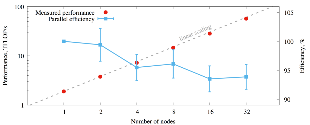
HPLinpack benchmark on the Colfax Cluster
Impact of System Configuration
Several boot-time settings in Intel Xeon Phi processors may impact the performance of calculations. They include the high-bandwidth memory mode (flat, cache or hybrid) and the cache clustering mode (all-to-all, quadrant, hemisphere, SNC-2 or SNC-4). We used the flat memory mode expecting the Intel MKL to automatically take advantage of the addressable high-bandwidth memory. We set the clustering mode to quadrant, which is optimal for most workloads. To validate our decision, we performed single-node (C=1) HPL benchmark in several other modes. As the table shown below demonstrates, the configuration that we picked indeed provides the best single-node performance. For multi-node runs, we expect the same configuration to be optimal.
| Mode | , GFLOP/s |
| Quadrant, flat | 1895 |
| Quadrant, cache | 1850 |
| All-to-all, flat | 1866 |
| SNC-4, flat (1 MPI process) | 703 |
| SNC-4, flat (4 MPI processes) | 332 |
Single-node HPL performance in various memory and cache modes.
Section 4. Summary
We presented the performance of the HPLinpack benchmark on the Colfax Cluster with up to 32 compute nodes. We also provided a simplified tuning methodology for HPL.dat.
The benchmark tuning parameters , , and are critical for achieving better performance. and must be chosen to make the grid square ( ) or almost square (
 ). We used the block size
  , which is the recommended value for Intel Xeon Phi processors 7250. The problem size is set to define the biggest problem that would fit into the available memory.
Our simplified tuning methodology yields acceptable results. For 32 nodes, the measured parallel efficiency  with =57~TFLOP/s. This amounts to 57/32=1.78~TFLOP/s per node. In comparison, according to the TOP500 list, the Intel S7200AP Cluster (Stampede-KNL) at the Texas Advanced Computing Center (TACC) achieves 842.9~TFLOP/s with 504 nodes, which amounts to 1.67~TFLOP/s per node.