FALCON Library: Fast Image Convolution in Neural Networks on Intel Architecture

We describe FALCON, an original open-source implementation of image convolution with a 3×3 filter based on Winograd’s minimal filtering algorithm. Compared to direct convolution, Winograd’s algorithm reduces the number of arithmetic operations at the cost of complicating the memory access pattern. This study is carried out in the context of image analysis in convolutional neural networks.
Our implementation combines C language code with BLAS function calls for general matrix-matrix multiplication. The code is optimized for Intel Xeon Phi processors x200 (formerly Knights Landing) with Intel Math Kernel Library (MKL) used for BLAS call to the SGEMM function.
To test the performance of FALCON in the context of machine learning, we benchmarked it for a set of image and filter sizes corresponding to the VGG Net architecture. In this test, FALCON achieves 10% greater overall performance than convolution from DNN primitives in Intel MKL. However, for some layers, FALCON is faster than MKL by 1.5x, but for other layers slower by as much as 4x. This indicates a possibility of a hybrid implementation with fast and direct convolution for a 30% speedup. High-bandwidth memory (MCDRAM) in Intel Xeon Phi x200 product family is a significant factor in the efficiency of the fast convolution algorithm.
Printable PDF: ![]() Colfax-Winograd-Summary.pdf (295 KB)
Colfax-Winograd-Summary.pdf (295 KB)
Code: github.com/ColfaxResearch/FALCON
Table of Contents
- Section 1. Convolution in Machine Learning
- Section 2. Winograd's Minimal FIR Filtering
- Section 3. Application to ConvNets
- Section 4. Transformation to GEMM
- Section 5. Implementation in Code
- Section 6. The FALCON Library
- Section 7. Performance
- Section 8. Conclusion
Section 1. Convolution in Machine Learning
Applications of deep neural networks (DNNs) to machine learning are diverse and promptly emerging, reaching the fields of assistive technologies, commerce, fundamental sciences, medical imaging and security (see, e.g., this article). DNNs thrive with abundant data. As a consequence, training DNNs often requires expensive development time and powerful computing resources. Therefore, even small improvements in the efficiency of the fundamental building blocks of DNNs can benefit the field of machine learning.
In image analysis with DNNs, one building block has gained particular importance in recent years: the operation of convolution of images with a filter. This operation is used in convolutional DNNs (ConvNets), which rely on the mathematical operation of convolution for position-independent object identification in images (see this article).
Numerically, convolution may be performed directly. This method is expensive in terms of computational complexity. For an image of size  and filter of size
  , direct convolution requires
 ") operations. However, arithmetic operations in direct convolution can easily be collapsed to form the general matrix-matrix multiplication (GEMM) pattern (see this article). This simplifies the design of convolution functions because the complexity of memory and cache traffic management is delegated to the implementation of GEMM. Efficient GEMM code exists in Basic Linear Algebra Subroutine (BLAS) libraries for nearly every computer architecture. In the case of Intel architecture, Intel Math Kernel Library (MKL) has highly efficient implementation of GEMM and of direct convolution expressed with matrix-matrix multiplication.
operations. However, arithmetic operations in direct convolution can easily be collapsed to form the general matrix-matrix multiplication (GEMM) pattern (see this article). This simplifies the design of convolution functions because the complexity of memory and cache traffic management is delegated to the implementation of GEMM. Efficient GEMM code exists in Basic Linear Algebra Subroutine (BLAS) libraries for nearly every computer architecture. In the case of Intel architecture, Intel Math Kernel Library (MKL) has highly efficient implementation of GEMM and of direct convolution expressed with matrix-matrix multiplication.
At the same time, it is possible to compute convolution with alternative methods that perform fewer arithmetic operations than the direct method. For example, fast Fourier transform (FFT) may be used to compute image convolution with complexity  \right)") (see this book). The asymptotic behavior of this algorithm predicts fewer operations than in direct method only if the filter is large enough:
(see this book). The asymptotic behavior of this algorithm predicts fewer operations than in direct method only if the filter is large enough: ") . However, this approach is not useful for ConvNets because they typically use filters as small as 2×2 or 3×3 pixels. In this range, the performance of the FFT method is poor compared to the direct method. In the domain of small filters, Winograd’s minimal filtering algorithm may be a better choice (see 1, 2). This approach has the same asymptotic complexity as the direct method, , but it reduces the number of operations by a constant factor. In this paper we present the implementation of convolution based on Winograd’s minimal filtering algorithm for a filter size
. However, this approach is not useful for ConvNets because they typically use filters as small as 2×2 or 3×3 pixels. In this range, the performance of the FFT method is poor compared to the direct method. In the domain of small filters, Winograd’s minimal filtering algorithm may be a better choice (see 1, 2). This approach has the same asymptotic complexity as the direct method, , but it reduces the number of operations by a constant factor. In this paper we present the implementation of convolution based on Winograd’s minimal filtering algorithm for a filter size  .
.
From here on, we refer to the convolution algorithm based on Winograd’s algorithm as “fast convolution”. This term, chosen by analogy with fast Fourier transform, signifies the algorithm performs fewer floating-point operations than the direct approach. At the same time, it is not trivial to implement a computer program performing “fast” convolution in less time than the direct method. This is because the fast algorithm requires data transformation with a complex memory access pattern, making it more difficult to express efficiently in code. The choice between an expensive yet simple algorithm (direct convolution) and less expensive but complicated algorithm (fast convolution) is not straightforward. It is difficult to predict, for instance, how well the hierarchy of memory and caches is able to serve the complex data access pattern of an algorithm based on strided or indirect memory access.
Section 2. Winograd’s Minimal FIR Filtering
The original Winograd’s algorithm is applied to the computation of finite impulse response (FIR) filters. Direct application of 2 consecutive steps of a 3-tap FIR filter with coefficients  to a set of 4 elements
  requires 6 additions and 6 multiplications:

The idea of Winograd’s method is to compute these two filter outputs as
 g_0,\\ m_2 = (d_1 + d_2) \frac{g_0 + g_1 + g_2}{2},\\m_3 = (d_1 - d_3) g_2,\\m_4 = (d_2 - d_1) \frac{g_0 - g_1 + g_2}{2},\\F_0 = m_1 + m_2 + m_3,\\F_1 = m_2 + m_3 - m_4.")
If we precompute the expressions /2") and
and /2") , then this procedure requires 8 additions and 4 multiplications, which is equal to number of floating point operations in the direct method. However, if our goal is to apply multiple filters gi to the same data di, then we can also precompute
, then this procedure requires 8 additions and 4 multiplications, which is equal to number of floating point operations in the direct method. However, if our goal is to apply multiple filters gi to the same data di, then we can also precompute ") ,
, ") ,
, ") and
and ") . With this done, the computation of F0 and F1 would only require 4 additions and 4 multiplications, yielding a speedup of (6+6)/(4+4)=1.5.
. With this done, the computation of F0 and F1 would only require 4 additions and 4 multiplications, yielding a speedup of (6+6)/(4+4)=1.5.
Section 3. Application to ConvNets
In the context of ConvNets, the operation of convolution applies a total of  filters of size to a batch of
  images of size
  with
with  channels in each. We enumerate filters with
  , and channels with
  . Each image we split into
 \times (W-2)/4") tiles and enumerate these tiles within the image with t, which ranges from
tiles and enumerate these tiles within the image with t, which ranges from  to
to  . The images within a batch are enumerated with n, which ranges from to .
Direct convolution of a  filter
  with a
  image
image  to generate a
  output tile
  requires
  multiplications and
  additions. As shown by Lavin and Gray, Winograd’s fast FIR filter computation can be generalized to 2D filters, which are mathematically similar to convolution. The fast method can be expressed as shown below:
![Y_{n,t,f,c} = A^{T}\left[ \left( B^{T}d_{n,t,c}B\right) \odot \left(G^{T}g_{c,f}G\right) \right]A](https://colfaxresearch.com/wp-content/latex/ee1/ee11e972b5c0bd5cc486bf0471363f9a-ffffff-000000-4.png "Y_{n,t,f,c} = A^{T}\left[ \left( B^{T}d_{n,t,c}B\right) \odot \left(G^{T}g_{c,f}G\right) \right]A")
where  is a matrix representing the image tile,
  is a
is a  matrix representing channel of filter , is a
  matrix with the output of the convolution of with ,

In the above equation, the symbol  indicates element-wise multiplication. Assuming that we have many image tiles and multiple filters, we can precompute transformed image tiles
 ") and transformed filters
and transformed filters ") . With that done, the algorithm requires
. With that done, the algorithm requires  multiplications between the transformed input and filters. For inverse transformations, 24 additions are required. This is already
 /(16+24)=1.8") times fewer operations than in the direct method. In addition to this, for the purposes of ConvNets, convolution must be applied to image channels, and results for individual channels must be summed:
times fewer operations than in the direct method. In addition to this, for the purposes of ConvNets, convolution must be applied to image channels, and results for individual channels must be summed:
![Y_{t,f} \equiv \sum_{c} Y_{n,t,f,c} = \sum_{c} A^T \left[ U_{n,t,c} \odot V_{c,f} \right] A.](https://colfaxresearch.com/wp-content/latex/f63/f63c3dc2e505e189d7612f74f019ada4-ffffff-000000-4.png "Y_{t,f} \equiv \sum_{c} Y_{n,t,f,c} = \sum_{c} A^T \left[ U_{n,t,c} \odot V_{c,f} \right] A.")
This allows one to perform the summation over channels first (16 additions per tile per channel) and apply inverse transformation after the summation,
![Y_{n,t,f} = A^T \left[ \sum_{c} U_{n,t,c} \odot V_{c,f} \right] A, \label{eq-sumfilters}](https://colfaxresearch.com/wp-content/latex/832/832f80dc0f254c1b78ccbd6fb1a76530-ffffff-000000-4.png "Y_{n,t,f} = A^T \left[ \sum_{c} U_{n,t,c} \odot V_{c,f} \right] A, \label{eq-sumfilters}")
thereby making its contribution to the operation count negligible. This results in net savings in the number of operations by a factor of /(16+16)=2.375") (we factored in the need to do 4 additions per channel in the direct method).
(we factored in the need to do 4 additions per channel in the direct method).
The expectation of speedup in the fast algorithm due to reduced number of operations hinges on the assumption that the precomputation of the forward and backward transformation of data takes little time. In reality, our experiments revealed that the straightforward implementation of the above algorithm does not provide high performance, and platform-specific optimization is required.
Section 4. Transformation to GEMM
In the above reasoning, we were making a silent assumption that the arithmetic throughput is the limiting factor of performance, i.e., memory traffic is completely overlapped with computation. This assumption holds true only if the order of tile convolutions is tuned to effectively re-use data in the processor’s caches. To avoid this complexity, as shown by Lavin and Gray, we we can express the arithmetic operations in the equations of the previous section as matrix multiplication, which allows us to delegate the complexity of overlapping memory traffic and computation to the GEMM function of a BLAS library.
Expressing the calculations through GEMM is possible because a transformed input tile  can be reused to multiply with multiple corresponding filter tiles, and, similarly, a transformed filter tile
  can be reused to multiply with corresponding input tiles across all the batches. In addition, the input and filter tiles that are multiplied across channels are accumulated into one output tile. Denoting the elements of the matrix as
  , and denoting elements of as
  , we can define a
  matrix
  with elements

For each pair ") , this equation expresses the multiplication of matrix
, this equation expresses the multiplication of matrix  by matrix
  . The final result of convolution can then be written as

To further improve performance, we collapse multiple matrices , which results in the first matrix in GEMM having greater number of rows.
Section 5. Implementation in Code
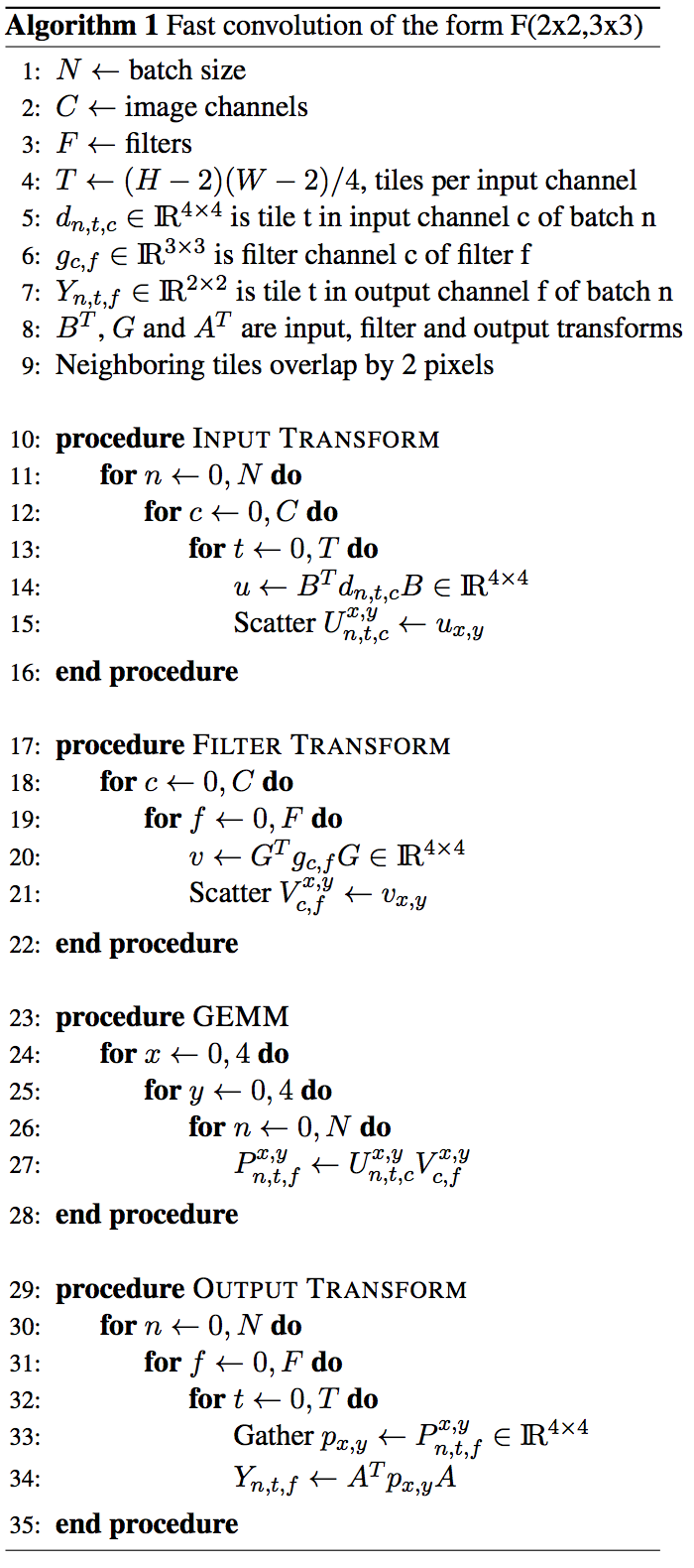
To compute convolution with the fast algorithm we follow approach similar to that shown by Lavin and Gray. There are three stages in this algorithm.
- Input transformation: scattering on the image and filter data sets to form the input matrices.
- Computation of product between transformed data and filter, and summation over channels expressed as GEMM, and
- Output transformation: gathering the elements from the product matrices and their transformation to form the actual output of the convolution
Data transformation and the procedure for expressing the computation with GEMM are explained thoroughly by Lavin and Gray. We have modified the data layout and way the input matrices for GEMM are formed and the pseudo codes shown below illustrate the procedure.
The input data format is flexible and can be tuned with the help of merge factor  to achieve high GEMM performance. Here,
  results in
  format,
  results in
  format, and
  shuffles and keeping
  as fixed inner dimensions.
Section 6. The FALCON Library
Our implementation of image convolution with a 3×3 filter, codenamed FALCON (FAst paralleL CONvolution) is available under the MIT license on GitHub. The code contains initialization and cleanup routines and a single interface function for performing a convolution. The syntax of the routines is described in the header file included in the GitHub repository.
The code of the initial implementation is optimized to perform with high efficiency on Intel Xeon Phi x200 product family (formerly Knights Landing). Optimization measures that ensure high efficiency in the transformation step include:
- Organizing the data structures in a way that, allows unit-stride access to input data and constant-stride access to output data;
- Tiling the loops to maximize register data re-use in cores;
- Unrolling inner loops to maximize the utilization of the register file and eliminate the dependence on the compiler estimate of the unroll factor;
- Automatically vectorizing inner loops with compiler hints;
- Tuning the count and affinity of OpenMP threads for maximum memory bandwidth;
- Placing scratch data in the high-bandwidth on-package memory of the Intel Xeon Phi processor;
- Tuning the inner dimension of data structures to be a multiple of 64 bytes (for aligned vector loads and stores), but not a multiple of 4096 bytes (to avoid cache associativity conflicts);
- Pre-allocating and re-using scratch data structures to avoid dynamic memory allocation in computation.
The code of the matrix multiplication step is optimized by:
- Using the BLAS implementation of single precision matrix-matrix multiplication (SGEMM), which in our tests was linked to the Intel Math Kernel library (MKL);
- Falling back to custom C language code instead of BLAS for tall and narrow (in column-major format) matrices, which are not handled efficiently by MKL;
- Fusing multiplication of multiple matrices with low row counts into a single larger GEMM;
- Using nested parallelism to process multiple matrix multiplications in parallel, with several threads working on each multiplication;
- Tuning thread affinity and using the “hot teams” functionality in Intel OpenMP to persist the affinity within inner thread teams across parallel regions.
We ensured the functionality of the code and tuned performance only for the hardware and software configuration described in the next section. Special attention was paid to optimize the performance of the code for convolution sizes used in VGG Net.
Section 7. Performance
Results reported here are obtained on a 68-core Intel Xeon Phi processor 7250 with 96 GiB of DDR4 RAM and 16 GiB of MCDRAM in flat mode. The system is running CentOS 7.2 with stock kernel. The code was compiled with Intel C compiler 17.0.0.098 (Build 20160721) and linked with Intel MKL 2017 (build date 20160802).
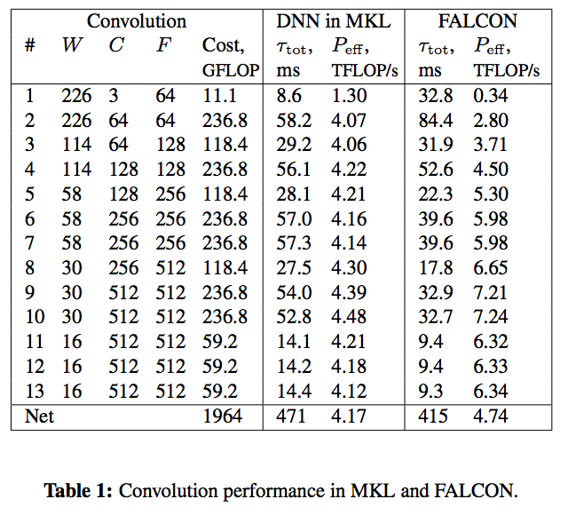
To benchmark the convolution routine, we opted to construct a benchmark based on a practical application: the forward pass of VGG Net. For that purpose, we built a driver application that performs and times convolutions for input sizes corresponding to the 13 layers of the VGG Net configuration D. We compare performance of FALCON with that of the convolution operation of the DNN primitives module of Intel MKL. We tested the performance with a batch size of  .
.
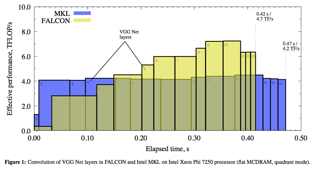
Our results are detailed in Table 1 and graphically presented in Figure 1. The x-axis in the plot is the time elapsed from the beginning of the calculation for a batch of input images. The y-axis is the effective performance of each layer in Intel MKL (blue rectanges with dashed outline) and FALCON (yellow rectangles with solid outline). Rectangles corresponding to different layers are labeled in their corners with numbers from 1 to 13. Effective performance is measured in TFLOP/s. It is computed as the ratio of the number of operations in direct convolution, estimated as (W-2)RSNCF") , to the measured wall clock time,
, to the measured wall clock time,  . Labels indicate the total time of processing of all layers (
 s for FALCON,
  s for MKL) and the corresponding effective performance (
 TFLOP/s for FALCON and
  TFLOP/s for MKL).
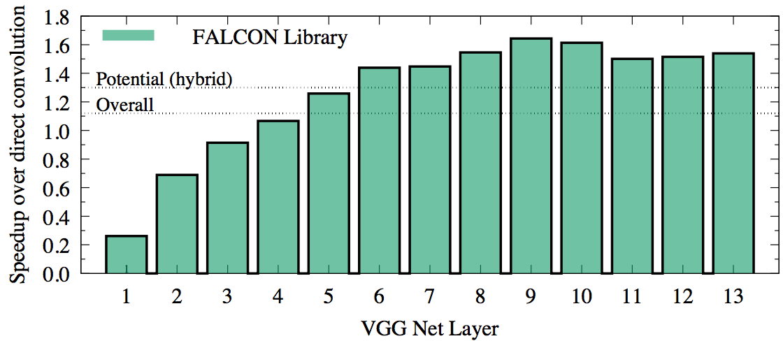
Details of Figure 1 show that the direct method used in Intel MKL performs better than FALCON for the first 3 layers. Indeed, the tall and skinny matrix used in these first three layers results in poor performance of GEMM in FALCON. However, starting from layer 4, the method based on Winograd’s algorithm used in FALCON is faster, and this performance advantage compensates for the time lost in the first three layers.
Based on the timing of MKL and FALCON performance, we argue that for specific DNN architectures, it may be possible to construct a hybrid convolution routine, in which for each layer either direct, or fast convolution is used, whichever is faster. In our example, using the direct method for the first 3 layers can save around  seconds, promising a total speedup over the direct method of
 \approx 1.3") .
.
Table 2 presents additional timing details. For each layer we report the time and effective bandwidth of input transformation  and output transformation
  . We also indicate the size
  and the performance of the GEMM used for filter application. Two sets of results are reported: with FALCON and the benchmark pinned to the high-bandwidth on-package memory (MCDRAM) and the on-platform memory (DDR4).
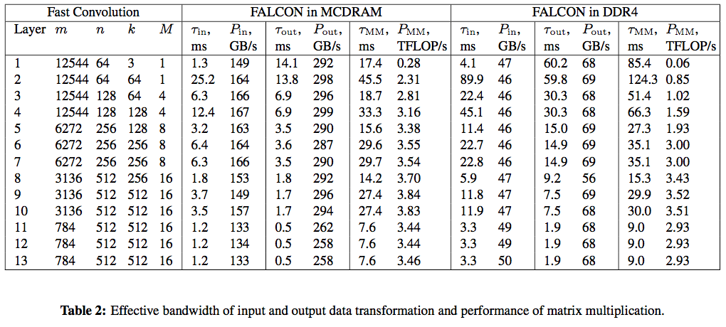
For high-bandwidth memory benchmarks, because our data structures were less than 16 GiB in size, we could fit them in the available MCDRAM. The processor was in flat memory mode, and so we ran the entire application in MCDRAM by setting the default NUMA policy with the numact tool (see “HOW Series: Knights Landing” for details). We also tested performance with the processor in the cache memory mode, and observed similar results. However, running the calculation in the on-platform memory (DDR4), we observed performance degradation by a factor of 2.5.
With MCDRAM, the input transformation achieves between 130 and 160 GB/s of memory access bandwidth. This is only around 30% of the bidirectional MCDRAM bandwidth. This is related to asymmetric traffic (more writes than reads), scattered memory pattern, and the presence of computation mixed in with data access. The output transformation achieves a better performance between 260 and 300 GB/s. In our experiments, the data layout that we ended up using optimizes the memory bandwidth as well as the overall timing.
The information about GEMM performance shows that with MCDRAM, it achieves between 3.2 and 3.8 TFLOP/s for layers 4-13, which is a large fraction of SGEMM performance in the ideal case of large square matrices (we measured 4.5 TFLOP/s). However, for layers 2 and 3, GEMM achieves only 2.3-2.8 TFLOP/s due to the small size of the inner matrix dimension,  . For layer 1,
  , and this computation is memory-bound. This is the case where we used custom C code instead of the BLAS call because in this case MKL delivered significantly worse GEMM performance.
Future optimization should focus the input transformation, as it operates at a low efficiency compared to its theoretical peak value. At the same time, the output transformation and GEMM are performing well. Poor performance in the first 3 layers may be ignored as MKL can be used in place of FALCON in this case.
Timing information in Table 2 shows that the memory-bound data transformation takes around 30% of execution time with the compute-bound GEMM taking the rest. We speculate that additional performance improvement may be obtained by splitting the batch of images into several sub-batches and overlapping in time the data transformation and GEMM computation.
Section 8. Conclusion
We presented the FALCON library, which implements fast convolution based on Winograd’s algorithm with performance optimization for Intel Xeon Phi processors x200 (formerly Knights Landing).
Performance Optimization
Even though Winograd’s minimal filtering algorithm reduces the number of floating-point operations necessary to compute convolution, it is not trivial to take advantage of these savings. Complex memory access pattern in input and output data transformations prompted us to carefully control data containers and memory access patterns in FALCON. Performing matrix multiplication also required thorough tuning by fusing smaller matrices into bigger ones, adjusting the strategy of multi-threading, and injecting custom code in place of BLAS routines in special cases.
High-Level Language
Despite the complexity of code optimization, the FALCON code does not use any assembly or intrinsic functions for explicit access to platform-specific instructions. Instead, it relies on automatic vectorization in the compiler, on standard functionality of the OpenMP framework, and on traditional BLAS routines. This simplifies future code maintenance and adaptation of the application to the upcoming computing platforms. Additionally, our case study proves by example the possibility of using high-level languages and frameworks in computational applications for Intel Xeon Phi processors.
Speedup over Direct Method
In the context of machine learning, we achieved convolution performance greater than that of the direct method implemented in the industry-leading mathematical library for Intel Xeon Phi processors. The performance advantage of approximately 10% was measured for a workload simulating VGG Net forward pass. Based on our argument for hybrid approach combining direct and fast algorithms (see Section 7), the speedup for this ConvNet may be improved to 30%. In some layers of VGG Net, FALCON is faster than MKL by as much as 50%, so the application of Winograd’s algorithm to convolution in other DNN architectures may yield even more significant speedups.
Importance of High-Bandwidth Memory
According to our comparison testing, high-bandwidth memory is the key element of the Intel Xeon Phi processor architecture that makes fast convolution perform better than the direct method. This is not an obvious result because ML tasks are generally considered compute-bound. However, as long as upcoming models of Intel Xeon Phi products retain the MCDRAM, they can benefit from fast convolution. In particular, performance advantage of fast convolution may develop strongly in the upcoming Knights Mill architecture specifically tuned for deep learning applications. In addition, the upcoming coprocessor form-factor of Intel Xeon Phi coprocessors is a suitable platform for ConvNets with fast convolution. Indeed, the data structures used for our VGG Net benchmark are under 16 GiB in size. This is suitable for offloading calculations to coprocessors, assuming that they are manufactured with at least the same amount of MCDRAM as their bootable counterparts.
Application to Machine Learning
To our knowledge, the FALCON library is the first open-source implementation of fast convolution for Intel Xeon Phi processors. We publish it under a permissive MIT license in hopes that the high-performance computing community can contribute to the improvement of the code and to its adoption in production machine learning libraries.
Modern machine learning frameworks are layered, exposing a DNN interface to the computer scientist, but delegating convolution to an intermediate layer, and relying on GEMM in the underlying BLAS library. Therefore, regardless of the complexity of the fast or hybrid convolution, as long as it is implemented in the intermediate layer, ML application developers are going to experience performance improvement all the while retaining their code and computing solutions.
Acknowledgements
We thank Alexander Heinecke (Intel) for his review that led to a bug fix in reported performance values.